Disclosure: Due to an NDA, I cannot show specific visual results or the source code of the model.

The global push for renewable energy and sustainable agriculture has sparked innovation at the intersection of these two critical sectors. One promising approach is agrivoltaics (AV), the practice of co-locating solar photovoltaic (PV) panels and agricultural crops on the same land. This synergy aims to optimize land use efficiency, generating clean energy while simultaneously producing food. However, a significant challenge, particularly in regions with less intense sunlight like the Netherlands, is the shading effect of solar panels, which can reduce crop yields.

Could supplemental lighting, specifically using efficient Light Emitting Diodes (LEDs), mitigate this shade effect and improve the overall financial viability of AV systems? To explore this complex question, a detailed simulation model was developed, as outlined in a recent consultancy report. This blog post dives into the architecture, assumptions, and insights derived from this modeling effort.

 

Unpacking the Agrivoltaic Simulation Model

The model, developed using the Python programming language, serves as a virtual laboratory to simulate the intricate dynamics of an AV system over a complete growing season. Its foundation is built upon the principles of the well-established LINTUL-1 crop growth model.

Core Mechanics:

1. Time Steps: The simulation progresses in discrete time steps, typically set at 90 seconds (τ=1/960 days), allowing for a detailed capture of daily environmental fluctuations and plant responses. This resolution was optimized to balance accuracy with computational efficiency.
2. Spatial Differentiation: Crucially, the model distinguishes between two distinct zones within the field: the area directly under the PV panels (shaded) and the area receiving unobstructed sunlight (sunlit). The proportion of each zone is determined by the panel_coverage parameter.

 

Simulating Growth: The Crop Module

At the heart of the model lies the calculation of biomass accumulation. This is done separately for the sunlit and shaded zones using a Radiation Use Efficiency (RUE) approach, adapted from the LINTUL model.

The potential biomass produced in a given time step (dW/dt) is calculated based on:

• Intercepted Photosynthetically Active Radiation (PAR).
• The crop’s specific RUE (how efficiently it converts light energy into biomass).
• The Leaf Area Index (LAI), which represents the amount of leaf area available to capture light.
• The light extinction coefficient (k), describing how light penetrates the canopy.

The formula used is:
dW/dt = DTR * f_PAR * RUE * (1 - e^(-k * LAI))
Different parameter sets (like RUE, specific leaf area (SLA), and biomass allocation fractions to leaves or yield) are used for the sunlit, shaded and LED-lit areas to account for potential plant adaptations to varying light levels. LAI itself is simulated dynamically, increasing as biomass is allocated to leaves, but capped at a maximum value (max_lai). In the shaded zone, LAI contributions from both the reduced sunlight and any supplemental LED light are tracked.

 

Illuminating the System: The Light and Energy Module

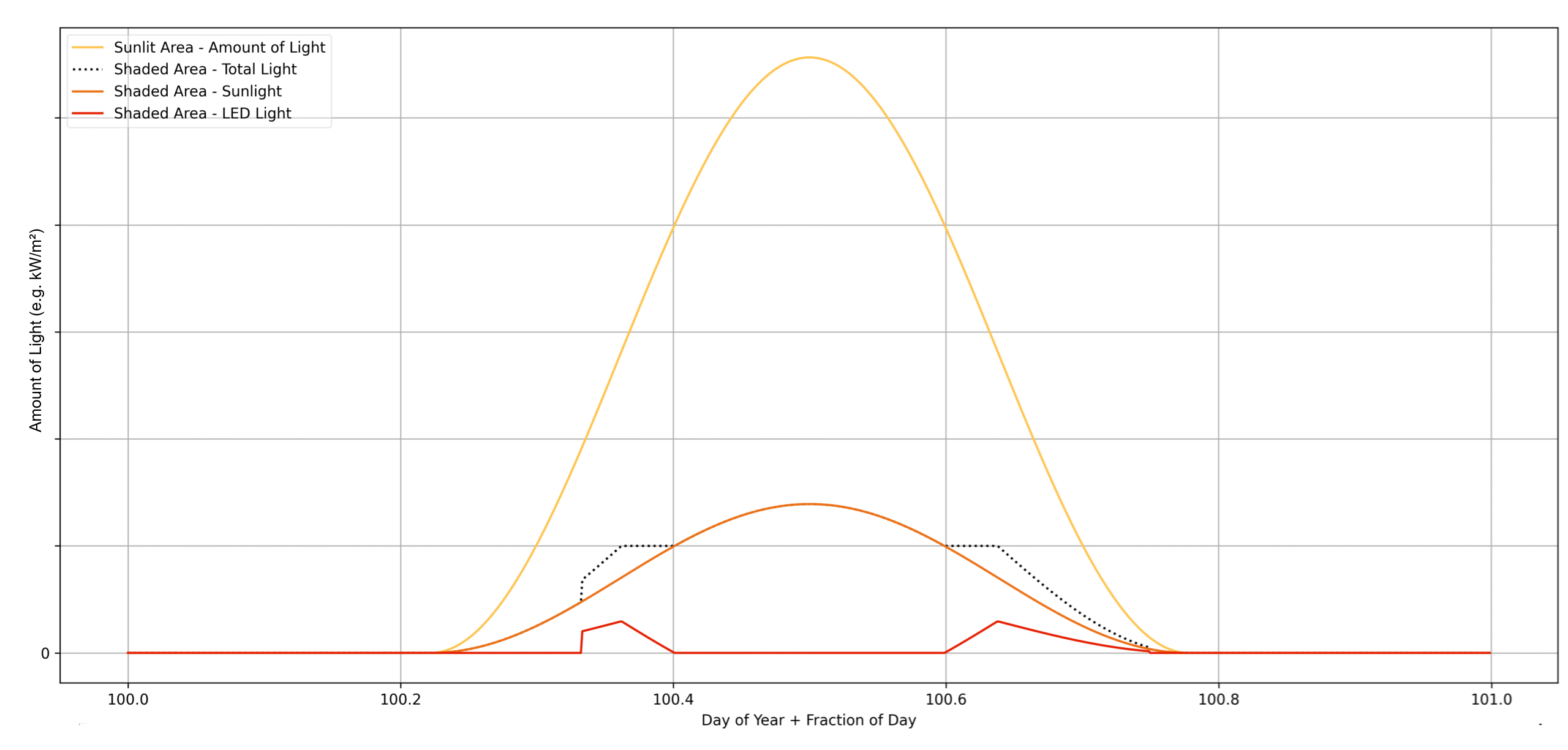
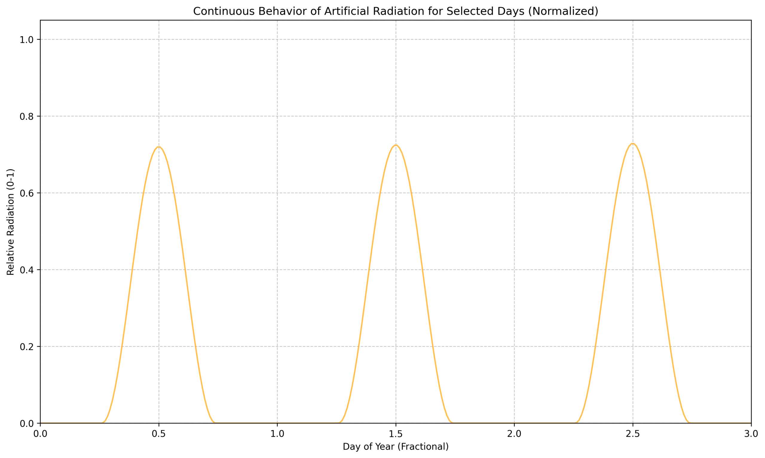
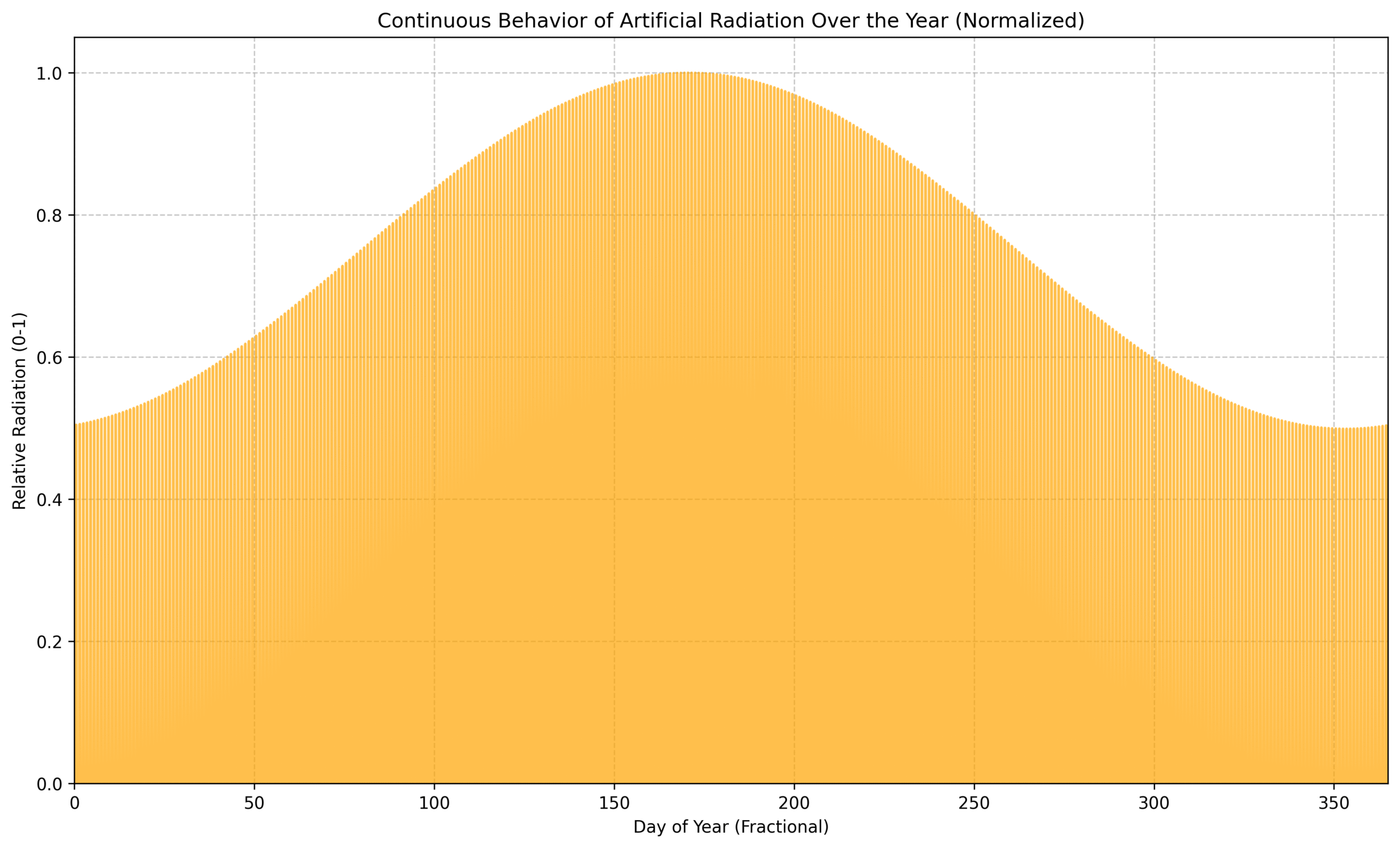
1. Sunlight Simulation: Incident solar radiation isn’t based on real-time weather but is estimated using a function that models daily and seasonal variations based on the day of the year and time of day (see Figures 2 and 3 at bottom). This provides the baseline light input for the sunlit area and, after reduction by a shaded_light_fraction, for the shaded area.
2. LED Supplementation: The model incorporates the potential use of LEDs in the shaded zones. LEDs can be scheduled to turn on during specific intervals. When active, the model calculates the LED light needed to supplement the existing shaded sunlight up to a target PAR intensity (led_light_amount_kWh_d_target). See limit of ‘Shaded Area – Total Light’ in Figure 1.
3. Energy Balance: Powering these LEDs requires energy. The model calculates the required electrical power based on the target light level and the led_efficiency. This demand is first met by the energy generated by the PV panels (calculated based on incident sunlight, panel_coverage, and panel_efficiency). If panel generation is insufficient, the model allows for the possibility of purchasing electricity from the grid (buy_energy_from_grid = True) at a specified price (grid_energy_price). If buying from the grid is disallowed (like in Figure 1), the LED light output is reduced proportionally to match the available panel energy (see LED curve [red] in Figure 1). Excess energy generated by the panels can be sold.

 

The Bottom Line: The Economic Module

Ultimately, the feasibility of any AV system hinges on economics. The model calculates:

• Total Crop Yield: Summing the biomass allocated to yield organs in both sunlit and shaded areas, converted to fresh weight using Dry Matter Content (DMC) values.
• Yield Profit: Multiplying the total fresh weight yield by the market price for the crop.
• Net Energy Profit: Calculating the revenue from selling excess energy minus the cost of any purchased grid energy.
• Total System Profit: The sum of yield profit and net energy profit.

 

Data, Assumptions, and Analysis

The model relies on specific input data: crop biophysical parameters (RUE, SLA, allocation fractions, etc.) are sourced from a separate data file (cases.csv), while economic and system parameters (prices, efficiencies, panel coverage) are defined within the main script.

Key Assumptions: It’s vital to understand the model’s underlying assumptions:

• Light: Simplified solar radiation curves, a constant PAR fraction (0.5), uniform shading under panels, and constant light extinction coefficients are assumed. Shadows are static.
• Crop Growth: RUE is assumed constant for a given condition (sunlit/shaded) and doesn’t vary with light intensity – meaning no light saturation effect is modeled. Biomass allocation fractions and SLA are fixed throughout the season. Growth is limited only by light via RUE, not by water, nutrients, temperature, etc.. No senescence is modeled beyond the LAI cap.
• LED System: LED light is treated as 100% PAR, applied uniformly based on a fixed schedule. Efficiencies (LED and panel) are constant. Energy is used or exported instantaneously (no battery storage).
• General: All parameters are constant throughout the simulation and assumed accurate.

 

Model Advantages and Limitations

Strengths:

• Simulates dynamic crop growth and energy flows throughout a season.
• Explicitly handles sunlit vs. shaded areas and potential crop adaptations.
• Integrates various LED lighting strategies and their energy costs.
• Allows crop-specific parameterization.
• Calculates key economic outputs.
• Includes tools for sensitivity and time-step optimization.

Weaknesses:

• Crucially, lacks modeling of photosynthetic light saturation.
• Assumes constant energy prices, ignoring real-world fluctuations.
• Uses fixed biomass allocation, unlike real plants where it changes with development.
• Assumes uniform conditions within zones, ignoring spatial variability and sun movement.

 

What Did the Sensitivity Analysis Reveal?

To understand which factors most influence the outcomes, a sensitivity analysis was performed. Key parameters were systematically varied around their baseline values, and the resulting changes in total yield and profit were measured and visualize using spider plots.

The analysis highlighted several critical factors:

• Panel Coverage: Increasing panel coverage logically decreases total yield but has a surprisingly linear impact on profit, suggesting energy revenue often outweighs yield profit changes in the scenarios tested.
• RUE: Radiation Use Efficiency, especially in the sunlit areas (rue), has a powerful, almost linear positive effect on both yield and profit. Interestingly, RUE in the shaded area (rue_shaded) had less impact, likely due to lower light levels and smaller shaded area in the default setup.
• Canopy Parameters (SLA & Allocation): Specific Leaf Area (sla) shows complex behavior, initially boosting yield but hitting diminishing returns as self-shading increases. Allocation to leaves accelerates canopy closure but faces similar limits, while allocation to yield is linearly linked to profit. These highlight the importance of partitioning strategies.
• Efficiencies: LED (led_efficiency) and Panel (panel_efficiency) efficiencies are critical drivers, particularly for profit. Higher LED efficiency significantly boosts the viability of supplemental lighting.
• LED Intensity: Increasing the target LED light amount shows non-linear effects, often plateauing when the system is limited by available panel energy (and grid purchase is off).

The Light Saturation Caveat: The model’s assumption of constant RUE (no light saturation) is a major consideration. Real plants don’t respond linearly to increasing light; their efficiency drops at higher intensities. This means the model likely overestimates growth under high light (direct sun or high LED levels) and may underestimate the benefit of LEDs when used to supplement low natural light levels.

 

Conclusion: A Tool for Exploration, Not a Crystal Ball

This agrivoltaic simulation model represents a valuable tool for exploring the complex interplay between crop physiology, solar energy generation, supplemental lighting, and economics in AV systems. Its ability to differentiate between sunlit and shaded zones and integrate LED strategies provides a framework for comparing different scenarios.

However, the model’s outputs must be interpreted with caution, primarily due to the simplifying assumptions made, especially the lack of a light saturation response and fixed biomass allocation. The sensitivity analysis clearly shows that outcomes are highly dependent on parameters like RUE and system efficiencies, emphasizing the need for accurate, site-specific, and crop-specific data.

While the model, in its current form and based on the tested parameters, suggests daytime LED supplementation faces significant economic hurdles due to energy opportunity costs, it lays the groundwork for future refinements. Incorporating light saturation curves and dynamic allocation would improve realism. Furthermore, the model highlights that strategies enhancing natural light penetration under panels without consuming electricity (like panel spacing or reflective materials) might be more immediately promising avenues for optimizing AV systems.

 

Future Improvements of the model

Significant enhancements to the model’s predictive accuracy and economic realism could be achieved by addressing two key limitations: the assumptions around light response and energy pricing. Firstly, incorporating a non-linear photosynthetic light response curve is crucial; the current model assumes constant Radiation Use Efficiency (RUE), which fails to capture light saturation (diminishing efficiency at high light intensities) and potential light inhibition, likely leading to overestimated yields under bright sun or strong LEDs and underestimated benefits in low-light supplementation scenarios. Secondly, integrating dynamic electricity pricing, reflecting real-world market fluctuations, would allow for a more sophisticated economic analysis, potentially unlocking strategies involving energy storage to buy or use power during low-price periods and sell during high-price periods, thus better evaluating the true cost-benefit of powering LEDs versus selling electricity.